Playing with ensemble models
Comparing prediction accuracy by model choice.

I’ve dabbled with ‘machine learning’ in three posts now Trump’s tweets, wine reviews and pub crawls, but never really put much thought into what effect the algorithm choice had on my predictions. In the following post I had a go at seeing what a prediction score looked like using a variety of machine learning methods.
The data I’m using is the Wisconsin Breast Cancer screening prediction model training set. This data has been around since the 90’s, and has been used countless times (it’s even a training set on kaggle). The data contains a number of metrics that were calculated from cell images. The ‘outcome’ is whether the cell is benign or malignant. 80% of the code for these models was written on a transatlantic flight - so for the most part, I have let the model tune itself over the default tuning grid. So - I make no promises it’s a fair comparison of the models, but it does represent how they perform on a relatively small dataset using (largely) the default tuning parameters.
The contender models
There are 27 families of machine learning models in Caret (one of several R packages for machine learning). I picked three that I understand, then tried out two methods of combing the three into ‘meta-models’.
In epidemiology we approach causal analyses first thinking about what are the clinically plausible variables that may confound our analysis. In prediction models, an epidemiologist is mainly worried about the functional form of the variables (e.g. is the effect of age linear), and the ramifications on the model assumptions. In machine learning, the same approach is taken for prediction models, but the vocabulary changes completely. Variable transformation, and to a certain degree model assumption checking, is called ‘feature building’. I did no ‘feature building’ in these analyses, beyond centering then scaling the data.
| The model | Description |
|---|---|
| Logistic regression (I’ll call it logistic) | Plain old logistic with all the variables banged in. Or more specifically, I used the ‘binomial’ family of glm(). |
| Generalized linear model via penalized maximum likelihood, aka GLMNet (I’ll call it elastic) | This model is a blend of ridge and LASSO. I allowed the model to scan the default Lambda, and it ended up picking a model that was leaning towards ridge regression over LASSO. |
| Random forest (I’ll call it … random forest) | An ensemble of trees! Again, letting the model scan over default mtrys. |
| Linear ensemble (I’ll call it … linear ensemble) | A meta-model, where the predictions from the logistic, elastic and random forest are combined using linear regression. |
| GBM ensemble (I’ll call it … GBM ensemble) | Another meta-model, but this time using a gradient boosted model to combine the component models (logistic, elastic and random forest). In vague terms, this model uses lots of weak learners, where the failures of the last model are weighted as important in the next model. |
In all models, cross validation came from 5 folds (for quick run times) repeated 3 times, and the candidate models were selected based on the AUC (area under the ROC curve).
Comparing the simple models
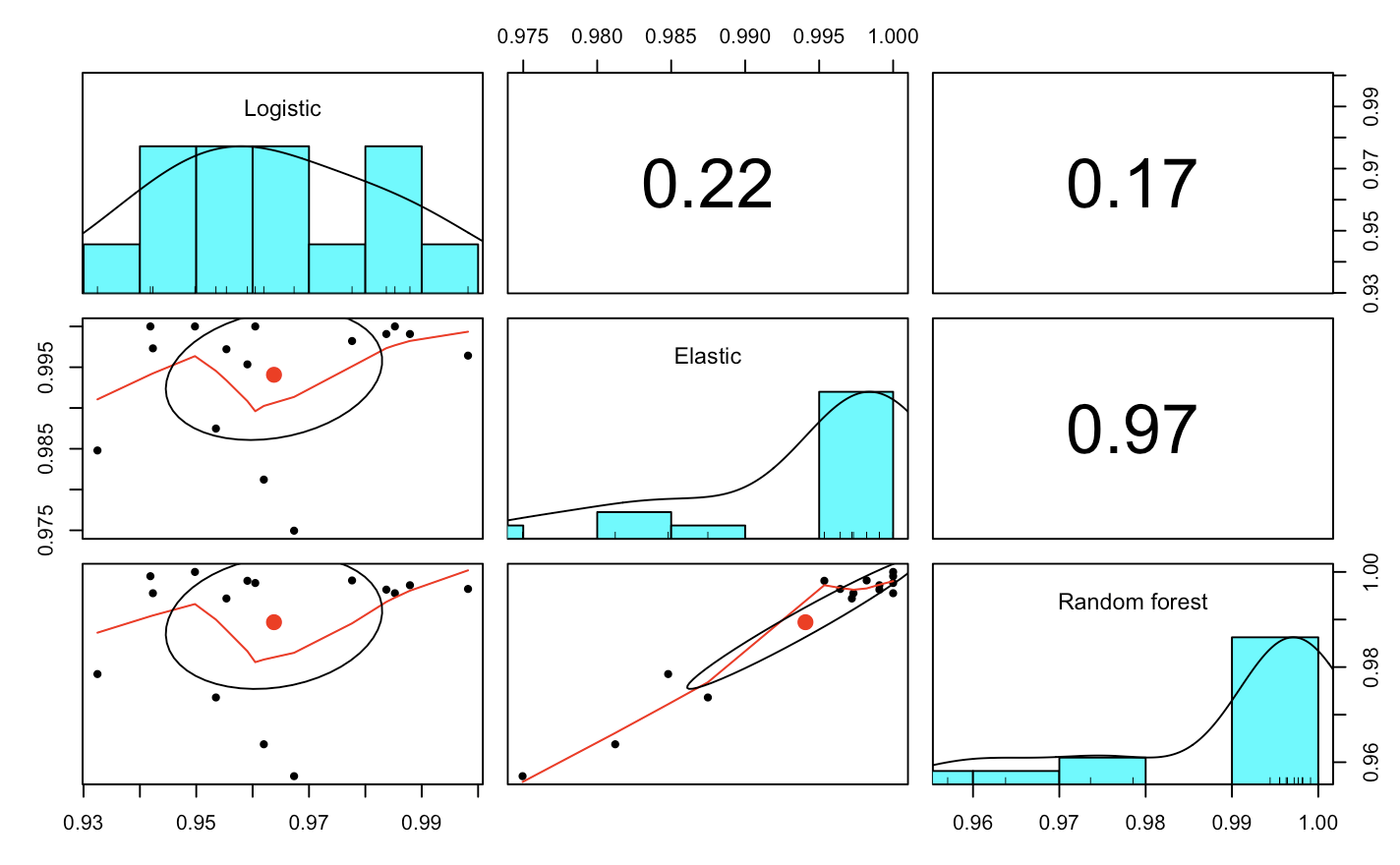
Between logistic, elastic and random forest, it was clear that the elastic model handled the data best. The variables were all continuous, and I have no evidence (I also haven’t looked) that there are threshold effects or weird functional forms that may have let the random forests shine. While it was a win here for the elastic - I’m not sure the results would be as clear if the data was less clean.
The key point when looking at the plots below is that the models were built to maximise the AUC. So the model that performed the best over a range of thresholds was selected - but when I predict on the model, by default it takes a probability of 0.5 as the cut point for deciding whether the model predicted the cell was benign or malignant. If I wanted to have a lower false negative rate, I could lower that threshold. This in turn would then mean there are more false positives. In a real analysis, I would have to involve clinical science, and decide on what balance of sensitivity vs specificity made more sense, considering that false positives and false negatives may have different ramifications.
In the plot below we see that the elastic and random forest models were strongly correlated across the folds. So where the random forest performed well, so did the elastic. The logistic model didn’t fare as well, but interestingly it looks like there was maybe one fold or two folds where the logistic model seemed to perform better than the two more advanced models (upper left quadrant of plots in left panels).
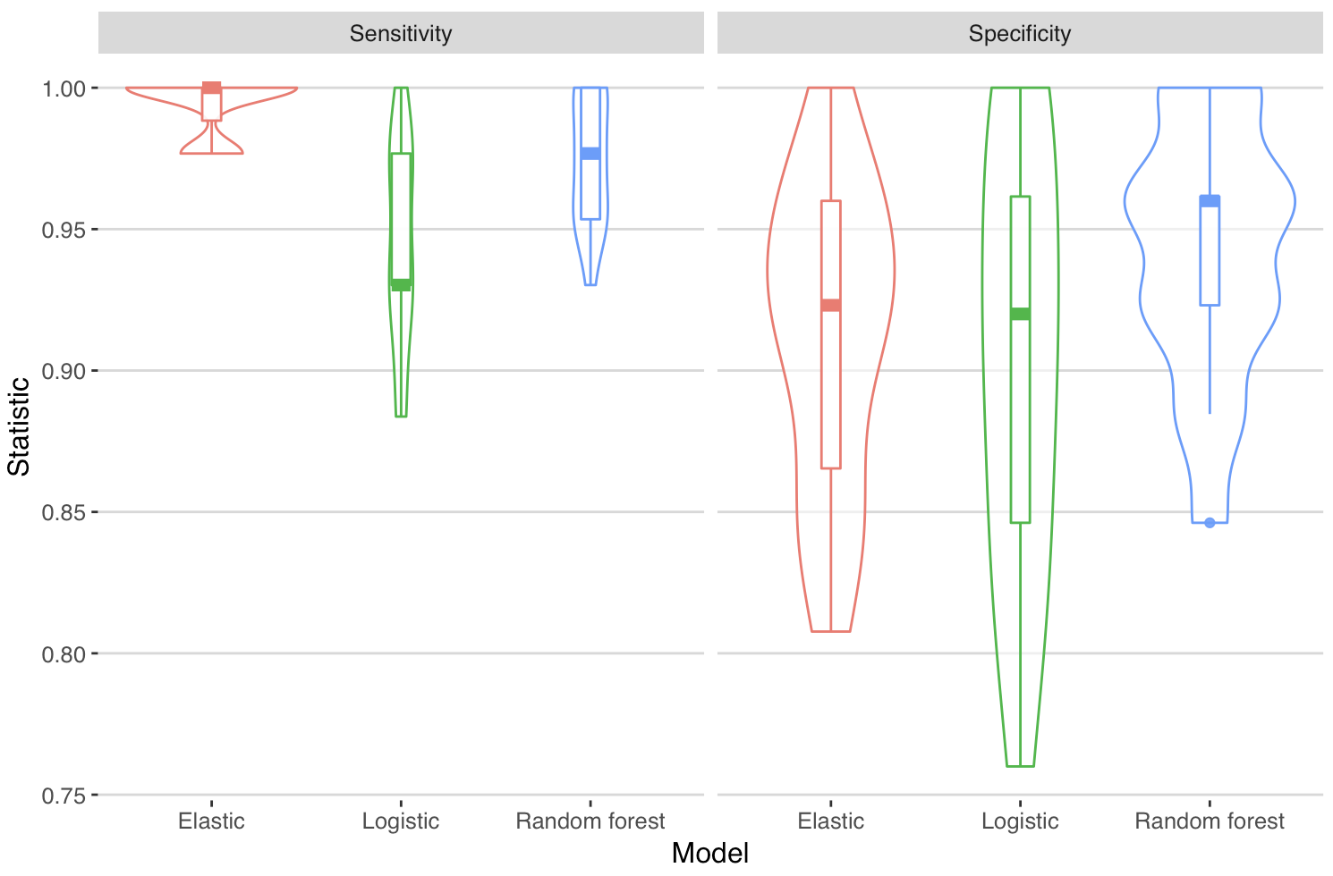
So - what about the specificity and sensitivity. Note that I have not considered what’s a clinically sensible balance of false positive to false negative, so this is simply the values derived from the default criteria of the models that had the largest AUC.
And, remembering this is a prediction model so any conclusions about causality are problematic, what variables present in the data independently contributed the most to the prediction? I was pretty surprised to see the differences here.
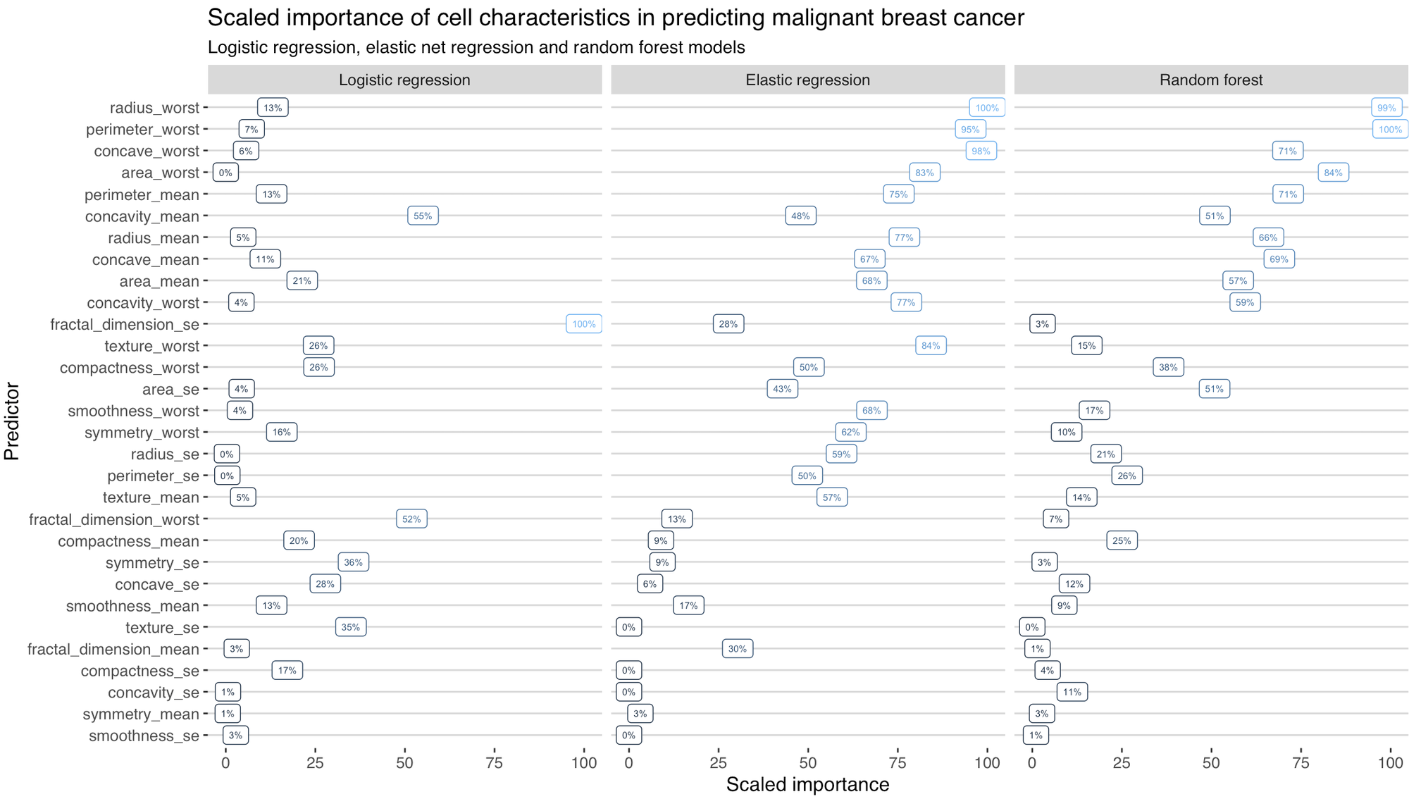
I should probably go back and look at the fractal_dimension_se variable to see why that was skewing predictions in the logistic model. Potentially the fact that I did not do any variable transformations or model checking (which is closely related to ‘feature engineering’ in ML speak) has amplified the poor performance of the logistic model.
Mix’n models
So I have three models. Maybe there are certain combinations where one model outperforms another. While technically speaking I already have an ensemble model (the random forest), I can go truly meta and create an ensemble of the previous three models.
A super simple way to build a meta-model would simply be to take a majority vote. I have three models, so in this binary prediction case I can take the prediction 2 or more models vote for. I’ll skip this though, as it is a pretty boring approach.
The first type of meta-model I made is the linear ensemble. My linear optimisation is just a glm model sitting on the predictions from the three base models. I actually tried getting really meta and running a ridge regression to build the ensemble, but it was out performed (within the testing data) by the linear model. As such, that foray into a ridge regression on a ridge has been discarded in favour of the simpler glm.
The last model I built is the GBM ensemble. This model uses stacking, where the predicted probabilities across 5 k-folds of the cross-validation from the original three models have been used to train a gradient boosted model. This GBM used trees as the weak learners.
Comparing all the models
Performance in the training data
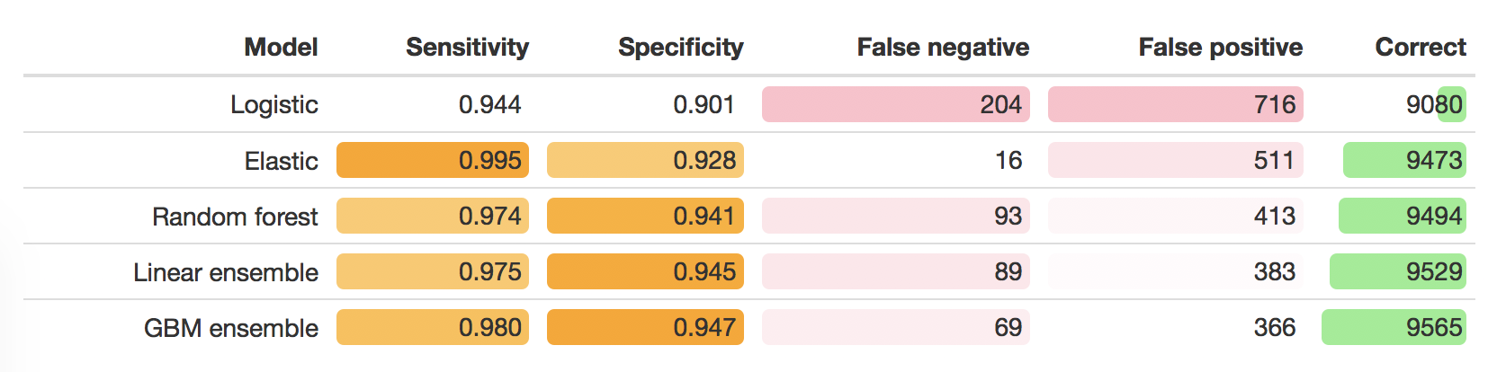
The following table shows the sensitivity and specificity of the models based on the cross-validation. To put those numbers in really simple terms, I applied those values to a theoretical population of 10,000 cell images, where the expected prevalence is the observed prevalence in the training data. This makes it obvious that the two ensemble meta-models get the most predictions correct, although that tradeoff between sensitivity and specificity present in the best performing model differs.
Performance on the test data
So far I have only looked at performance in the training data. I also set aside 40% of the data as a testing set - which means I can now take the models trained on 60% of the data, and see how they fare on that last 40%.
I was really surprised by the lack of correlation between the cross-validation (in training data performance) and the test data performance. I only did 5 k-folds, but even when rerunning with 10 the result was consistent. In the table below we see, unlike what is expected from the performance in the training data, the elastic performed best - suggesting that improving the model within the training data by building an ensemble model, actually led to a model that had degraded performance in the test data.
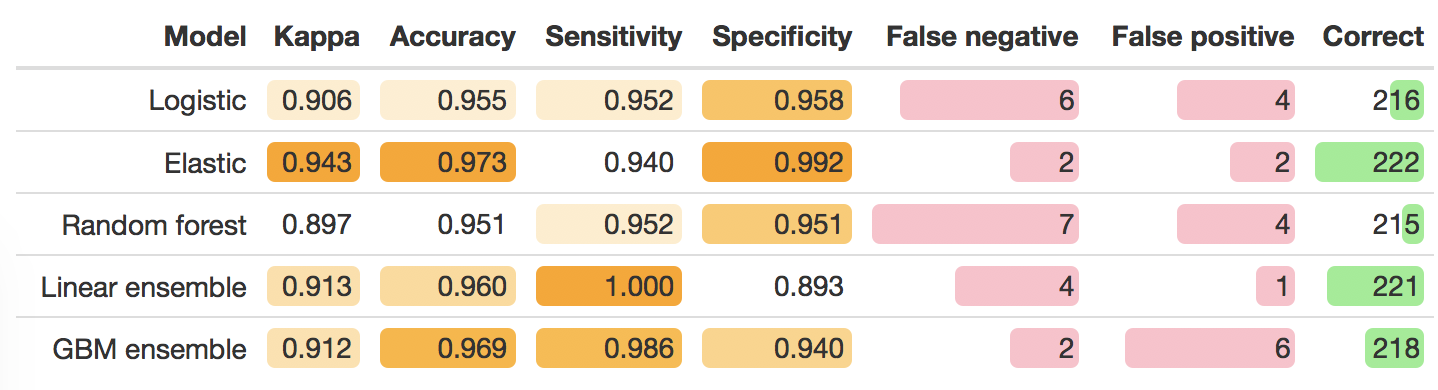
My first impressions is that the elastic model, which has a some nifty rules to filter out variables and build a parsimonious model, has also managed to build a model that is the most immune to overfitting - which in turn leads to it performing better in the test data. Conversely - I only invested a couple of hours to go from the raw data to having 5 models - so potentially I’ve simply identified a model that performs well when someone does some recreational/educational model building. I would need to carefully work through each step tuning the model to be in a more robust position to differentiate which model suited this prediction question best.
James Black
PhD (Cantab)
James Black. Kiwi | Epidemiologist | Data Scientist | Engineering enthusiast.