Tina and I recently moved into a new apartment in Basel. Currently, our walls are completely bare - so I thought it would be cool to use the Google maps API to try and make a wall hanging based off Basel location data. I’ve wrapped up all the code to make these plots in a function, and details on how to run the code is here.
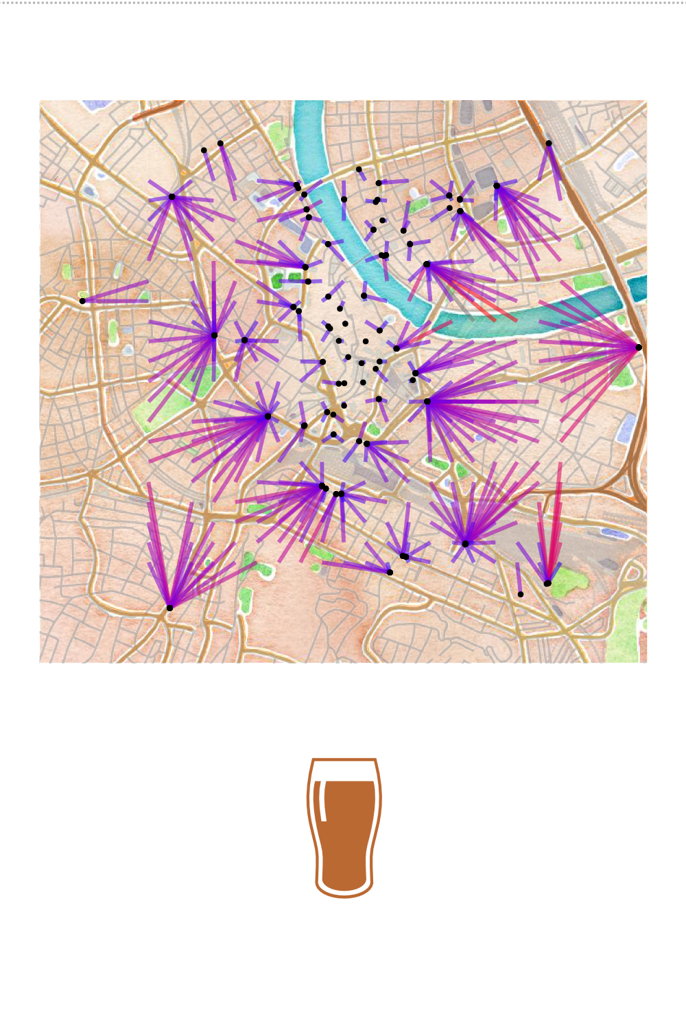
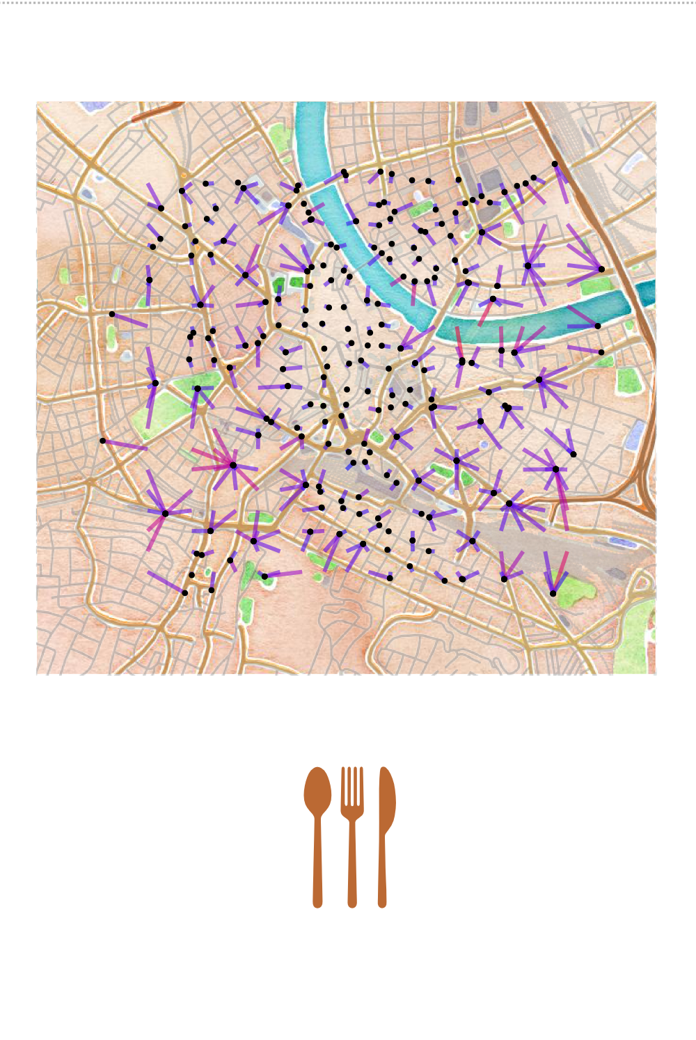
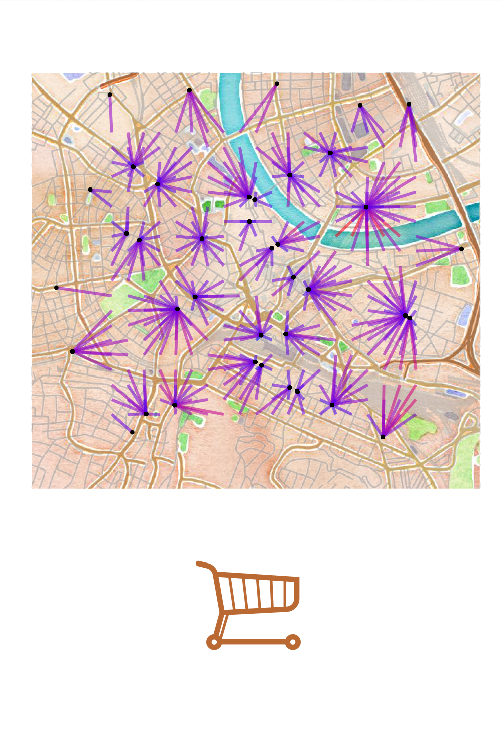
The final result is this.

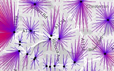
And a close up..


Which I made with this code…
Variables that change
Below are the master inputs that need to be set. This can easily be edited for more specific searches. For example, in the supermarket plot above, I added in name=coop|migros to limit the search to only the two major supermarket chains (so no budget or ethnic supermarkets are in that plot).
# Variables to input
  google_key <- "YOUR_GOOGLE_API_KEY"
  # bounding box limits for map
  top_lat <- 47.565
  bottom_lat <- 47.54
  left_lng <- 7.57
  right_lng <- 7.61
  zoom_level=13 # resolution of map
  # steps for grid
  steps = 20
  # thing to search for
  type=bar
  # see link for full list
  # https://developers.google.com/places/supported_types
{% endhighlight %}

## Functions

### Pull nearest amenity

This function will take the location frame you give it, make a grid (the number of points defined by `steps`) and get the closest type of place you are looking for.

{% highlight r %}
jb_pullnearby <- function(
  GOOGLE_API_KEY = google_key,
  # Map corners
  lat_NW = 47.56232,
  lng_NW = 7.57373,
  lat_SE = 47.54263,
  lng_SE = 7.60274,
  steps=100,
  type="restaurant"
){
  library(jsonlite)
  library(dplyr)

  # 100 steps left and 100 down
  lat_incr = (lat_SE-lat_NW)/steps
  lng_incr = (lng_SE-lng_NW)/steps
  # Start in the northwest and iterate to the southeast
  lat_curr = lat_NW
  lng_curr = lng_NW

  # clear output
  data_output <- NULL

  # Open loop

  for(i_lat in 1:steps){
    for(i_lng in 1:steps){
      # current location
      curr_location = paste0(lat_curr,",",lng_curr)
      # url to call api
      url <- paste0('https://maps.googleapis.com/maps/api/place/nearbysearch/json?location=',
                    curr_location,
                    '&key=',
                    GOOGLE_API_KEY,
                    '&rankby=distance&types=',
                    type)
      response <- fromJSON(txt=url)$results
      if(!is.null(nrow(response))){
      temp_location <- response$geometry$location
      temp_info <- response %>%
        select(place_id,icon,name,vicinity)
      temp_data <- cbind(temp_location,temp_info)
      # Make line of data from response
        # note rankby means sorted by proxomity!
      temp_data <- temp_data %>%
        mutate(
          n = 1:n(),
          loc_lat = lat,
          loc_lng = lng,
          lat = lat_curr,
          lng = lng_curr,
          i_lat = i_lat,
          i_lng = i_lng
        )
      # add data
      data_output <- rbind(data_output,temp_data)
      }
      # Move along one lng increment
      lng_curr <- lng_curr+lng_incr
    } # longitiude loop
    # reset longitude
    lng_curr = lng_NW
    # Move along one lat increment
    lat_curr <- lat_curr+lat_incr
  } # latitude loop
  return(data_output)
} # close function
Get walking time and distance
This function will take two locations and get back the walking time and distance from Google.
jb_googledist <- function(
  origin=paste0(lat,",",lng),
  destination=paste0(lat,",",lng),
  GOOGLE_API_KEY=google_key){
  library(XML)
  library(RCurl)
  xml.url <- paste0(
    'https://maps.googleapis.com/maps/api/distancematrix/xml?origins=',
    origin,'&destinations=',
    destination,
    '&mode=walking&key=',
    GOOGLE_API_KEY,
    '&sensor=false')
  xmlfile <- xmlParse(getURL(xml.url))
  time <- xmlValue(xmlChildren(xpathApply(xmlfile,"//duration")[[1]])$value)
  time <- round(as.numeric(time)/60,1)
  dist <- xmlValue(xmlChildren(xpathApply(xmlfile,"//distance")[[1]])$value)
  distance <- as.numeric(dist)
  output <- data.frame(time=time,distance=distance)
  return(output)
}
Run functions and plot
This final code is an example of how to use the two functions to make a plot like the three above. The first code block (with the changing inputs needs to also be run, as this code uses those inputs).
# Get the nearest
data_locations <- jb_pullnearby(
  GOOGLE_API_KEY = google_key,
  # Map corners
  lat_NW = top_lat,
  lng_NW = left_lng,
  lat_SE = bottom_lat,
  lng_SE = right_lng,
  steps=steps,
  type=type
)

  # Drop to closest restaurant
  dataset <- data_locations %>%
    filter(n==1)

# Get google distance
  # empty results df
  dataset_distances <- NULL
  # start loop over data
  for(i in 1:nrow(dataset)){
    # current iteration
    i_origin = paste0(dataset$lat[i],",",dataset$lng[i])
    i_destination = paste0(dataset$loc_lat[i],",",dataset$loc_lng[i])
    # get distances
    i_distance <- jb_googledist(
      origin=i_origin,
      destination=i_destination,
      GOOGLE_API_KEY = google_key)
    # load into data
    dataset_distances <- rbind(dataset_distances,i_distance)
  }
  # add to data
  dataset <- cbind(dataset,dataset_distances)

# map it
library(ggmap)
  ## get the map from stamen
  basemap <- get_stamenmap(
    bbox = c(left = left_lng,
             bottom = bottom_lat,
             right = right_lng,
             top = top_lat),
    zoom=zoom_level, source='stamen',crop = TRUE,
    maptype="terrain-lines", color="bw")

  # Order points high to low
  dataset <- dataset[order(-dataset$distance),]

# Plot - pubs
  ggmap(basemap,extent = 'device') +
    geom_segment(
      aes(x=lng, xend=loc_lng,
          y=lat, yend=loc_lat,
          colour=distance,
          alpha=0.5),
      size=2, data=dataset) +
    scale_colour_gradient(limits=c(0, 2500),
                          low="blue", high="red")+
    geom_point(aes(x=dataset$loc_lng,
                   y=dataset$loc_lat),size=3)

  ggsave("map.svg", width=10, height=10)